Binomial Distribution

This entry explores binomial distribution. We shall explore the binomial distribution, conditions for a binomial distribution, binomial cumulative distribution function, mean and variance of a binomial distribution. Before attempting this section you must have good knowledge of the factorial notation and how to use binomial expansion.
The following are key points and formulae you will learn towards the end.

Finding probabilities using binomial theorem

First we shall explore how to use binomial theorem to find probabilities.

Example

A biased coin is to be thrown 10 times. Let p be the probability that the coin lands on heads when thrown. Find the probability of the coin landing heads;

1. 10 times
2. 6 times
3. 3 times

Let us find the probability of the coin landing heads 10 times when thrown 10 times.
We know the probability of getting heads is p. Here we assume that each throw is independent so we can simply multiply the probabilities at each throw together to obtain the probability when the thrown 10 times.

Now we shall find the probability of landing heads when thrown 6 times;
When the coin does not land heads it must land tails. Here we shall let q = probability of landing tails. The coin can only land on heads or tails so we have a fixed number of probabilities. The number of arrangements with a total of 10 objects with 6 of which are unique can be written as the following. This is from the factorial notation <-[LINK]
…so there is 210 number of arrangements of 6 heads and 4 tails. Therefore using the same idea as above p⁶ for the 6 heads, q⁴ for the 4 tails, so we have the expression as;

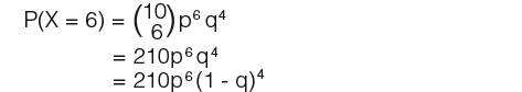
Notice that q is (1 – p). The probability of getting tails is the probability of not getting heads and we know probabilities always add up to 1 and not less than 0. Therefore (1 – p) = q.
Lastly the probability of landing heads when thrown 3 times, that is;

Notice that the probabilities above are terms in the following binomial expansion;

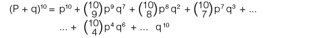
You could use the full binomial expansion to write down the probability distribution for the random variable X.

When is a binomial distribution a suitable model

In the above example there were 4 conditions explored for binomial distribution. We shall list the conditions here;

• A fixed number of trails, n

  A binomial distribution is suitable when there is a fixed number of trials. In the above example the coin was thrown 10 times. So n=10 was fixed.

• Each trail should be success or failure

  The distribution is called binomial because there are only 2 cases for each trial. In the above example each throw could land on heads (H) or tails (T)

• The trials are independent

  The trials must be independent i.e you must be able to multiply the probabilities together.

• The probability of success, p at each trail must be constant

  In the above example we assumed that the probability was p at each throw.

If the above conditions are satisfied we say that the random variable X ( = the number of success in n trials) has a binomial distribution which can be written as;

…where…

• ’B’ for binomial
• n for the number of trials
• p for the probability of success at each trial

…then…

n is often referred to as the index and the parameter of the binomial distribution.
Below we shall look at some examples using the equation above.